FEA Simulation Setup: A Simple Overview

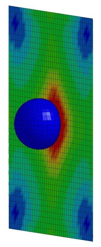
In this guide, I’ll explain the process of setting up and simulating a finite element analysis (FEA) model using boundary conditions, much like what you’d see in real-life scenarios. When I think of FEA simulations, this is what comes to mind.

So, what does a heat map actually represent? What loading conditions were applied to create it, and how can we use the results? Such visualizations can be achieved using FE software like LS-DYNA, ANSYS, or ABAQUS, often referred to as ‘solvers’ since they solve the complex scenarios we define.

Pre-Processor

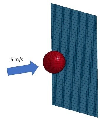
Simulations like the one I demonstrated are set up using a pre-processor, where you specify how to ‘test’ or manipulate your model. While each solver may come with a built-in pre-processor, it’s helpful to view each step—pre-processing, solving, and post-processing—as distinct parts of the process. Here, I’ll use the LS-DYNA framework as an example, though this applies to any FE software. LS-DYNA’s pre-processor, LS-PrePost, acts as both a pre- and post-processor, as the name suggests. This is where you define material properties, prescribe motions, set model constraints, or even create boundary conditions like an impactor.

For instance, imagine a ball moving at 5 m/s toward a section of sheet metal. The ball’s material properties are set to elastic, like rubber, while the wall is defined as material representing aluminum. A contact is established between the ball and the wall, and the wall’s edges are constrained in all directions, allowing the inner area to flex upon impact. In the pre-processor, you can also specify details such as the simulation duration and the outputs you want—similar to using sensors like accelerometers in real-world testing. This step is crucial; after all, what’s the point of running a complex simulation if you don’t have data to analyze afterward?

Solver

Once everything’s set up, the solver processes the inputs and solves the problem over time, calculating things like the ball’s deformation upon impact, the stress on the wall, and the ball’s rebound velocity. Solvers make this manageable by breaking the problem into small elements and combining their solutions.

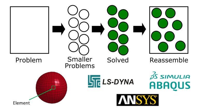
Solvers make our work much easier by handling the calculations for hundreds or even thousands of elements over time—something that would be impractical by hand. The time needed to complete a simulation can vary widely based on its complexity, duration, and the computer’s processing power. Some simulations can take days or even weeks to finish, often requiring powerful servers with dozens of processors rather than personal computers.

Post-Processor

Once the simulation is complete, the post-processor can be used to view the output animations and analyze data. Results may be available as ASCII files that can be loaded into LS-PrePost’s post tab, where you can plot details like the trajectory of a rubber ball or the impact force against a wall. The fringe tab can also display a stress heat map on the wall, similar to what we saw earlier.

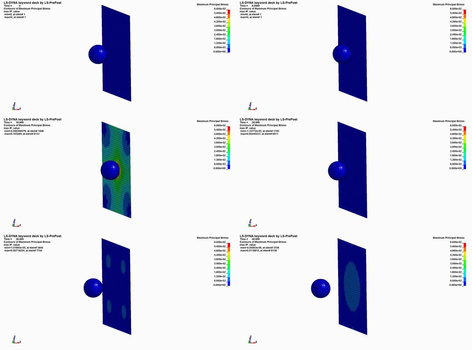
It’s crucial to use FE simulation data effectively, as these insights can reveal issues that might otherwise go undetected. For instance, an automotive manufacturer could identify stress concentrations at a joint in a vehicle frame, preventing potential failures. FE simulations can save lives and reduce costs by minimizing the need for extensive physical testing.

To summarize, running an FE simulation involves three main steps: setting up in a pre-processor, running the simulation with a solver, and analyzing data in a post-processor.

Have a question or comment? Join the discussion here.